Laboratory
-
sp-ICP-MS
Principle -
sp-ICP-MS
Sample Prep. -
sp-ICP-MS Measurement
-
sp-ICP-MS
Data Analysis
Summary of Analytical Technique
Single particle Inductively Coupled Plasma Mass Spectrometry (sp-ICP-MS) is a special type of Inductively Coupled Plasma Mass Spectrometry (ICP-MS) technique developed for the characterization (diameter, composition, etc.) of individual nanoparticles (NPs) in suspension. By flowing a solution containing single NPs or agglomerates at an appropriate concentration (about 106 particles/mL) into an inductively coupled plasma (6000-10000 K), each NP produces an ion cloud that causes a pulse of the mass signal related to the diameter of a NP. sp-ICP-MS overcome the limitations of electron microscopy requiring dry samples, by directly analyzing NPs in liquid suspensions, providing composition, mass, and diameter information for thousands of NPs per minutes. Moreover, by directly measuring the mass of each NP, sp-ICP-MS minimizes environmental parameters (e.g., temperature and vibration) often observed in other NP characterization methods based on the Brownian motion of NPs, such as NTA and DLS.
Principle of Analytical Technique
sp-ICP-MS is based on conventional ICP-MS which consists of ionization process, sample introduction system, mass spectrometer and detector. The basic principles of ICP-MS are as follows:
Ionization process
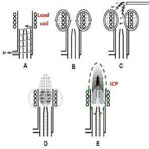
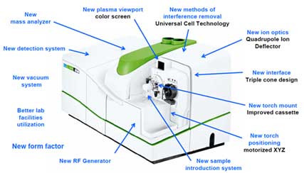
The Inductively Coupled Plasma (ICP) is a module for ionization by making high temperature of plasma. The plasma is generated by combining Ar gas flowing through a series of concentric quartz tubes (the ICP torch) and an induction coil whose energy is supplied by a radio-frequency (RF) generator. Specifically, flowing argon gas is initially ionized by sparks from a Tesla coil. The resulting argon ions and electrons interact with a fluctuating magnetic field generated by the induction coil by the RF generator that radiates 0.5 to 2 kW of power at 27.12 MHz or 40.68 MHz [6]. This interaction causes argon ions and electrons to flow in circular paths within the coil shown in Figure 1B. The resistance of argon ions and electrons to this charge flow causes ohmic heating of the plasma having a temperature of about 6000K. Since the plasma temperature is very high, it is necessary to insulate the outer quartz cylinder. Thus, thermal isolation of the outer quartz cylinder is achieved by flowing argon gas tangentially around the wall of the tube as indicated by the arrows in Figure 1A.
Sample introduction system
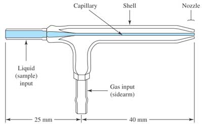
When a liquid sample enters the instrument, through a peristaltic pump, the aerosol of find droplets are generated by a meinhard nebulizer (see Figure 2). During the introduction into the plasma, the liquid droplets, containing the analyte sample is dried to a solid and then heated with gas to form atoms in the analyte. During passing through the plasma, the atoms of the analyte absorb more energy and eventually release one electron to form singly charged ions. These singly charged ions exit the plasma and enter the interface region to focus before going to the mass spectrometer system. The interface region, consisting of triple cones (sampler cone, skimmer cone, hyper skimmer cone), is the connection between the plasma region (operating atmospheric pressure) and the mass spectrometer (operating at very low pressure of 10`-8 bar).
Mass spectrometer and detection
Mass spectrometer can separate singly charged ions from each other by elemental mass. Commercial ICP-MS systems use three main types of mass spectrometers: quadrupole, time-of-flight, and magnetic sector. On NEXION 300D instrument, the mass spectrometer is quadrupole. Under the control of the instrument software, the mass spectrometer can move to m/z necessary to measure the elements of interest in the analyzed sample. After separation by the mass spectrometer, the selected ions hit the active surface of the detector and generate measurable electronic signals.
Difference between conventional ICP-MS and sp-ICP-MS
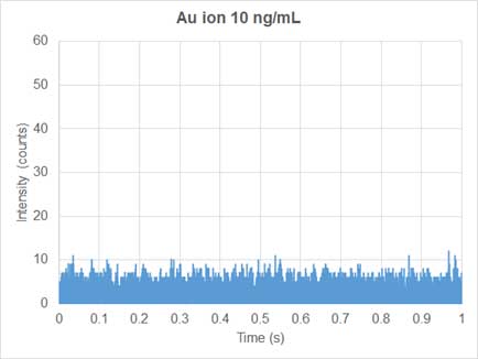
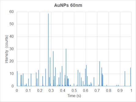
Conventional ICP-MS is used for quantifying dissolved ions in samples. Since the ions are homogeneously distributed in the dissolved ion samples, the mass signal of the dissolved elements entering the plasma and traveling to the detector per unit time, is relatively constant. Thus, the generatein the nanoparticle solutd ions produce a continuous signal over time (Figure 3). In sp-ICP-MS, on the other hand, suspension solution of nanoparticles enters the system and the mass signal is not continuous (Figure 4). Each nanoparticle is ionized to produce an ion cloud. Each ion cloud produces a signal pulse, so the signal in the nanoparticles solution has many peaks equivalent to many nanoparticles (Figure 4).
Two important time-related terms in sp-ICP-MS are “dwell time” and “settling time”. According to Chady et al [5], the time it takes for a detector (e.g. quadrupole) to analyze each m/z before moving on the next m/z is called "dwell time". After each dwell time measurement, the electronics need some time to stabilize before the next measurement. This stabilization time is called “settling time" and is overhead and processing time.
Taking into account the effect of dwell time and settling time during ICP-MS measurements, some signals may be lost at settling time. In the case of dissolved ions in conventional ICP-MS, this loss is not significant, since the solution is homogeneous and the signal is continuous. For nanoparticle suspension solutions of sp-ICP-MS, this loss is significant due to the discrete signals of the nanoparticles (Figure 4). On NEXION 300D, the settling time is zero, minimizing the losses mentioned above.
Theory of sp-ICP-MS
sp-ICP-MS, assumes that each single particle produces a signal pulse called particle event, under three conditions(Figure 3): 1)the dwell time is short so that one or more particle event do not overlap; 2) the flow rate of nanoparticle suspension solution is constant; 3) the nanoparticle suspension solution has a low particle concentration so that multiple nanoparticles do not overlap within one dwell time period. If the assumption is correct, number concentration of nanoparticles (particles/mL) is directly related to the frequency of the pulse as shown in the following equation [6].
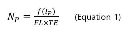
, where Np is the particle concentration (particles/mL), f(IP) is the frequency of particle events (number of pulses/min), FL is the sample flow rate (mL/min) and TE is the transport efficiency (%). The suspension solution of sample is introduced into the plasma by the meinhard nebulizer producing fine droplets. Only a small fraction (<20 %) of total number of droplets reaches the plasma. This ratio is called transport efficiency (TE). Transport efficiency is needed to calculate the particle concentration (number) of sample.
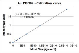
sp-ICP-MS measures the pulse signal of nanoparticles. In order to relate pulse to the diameter of nanoparticles, calibration curves of intensity - particle mass and mass-diameter equations are used. First, we need to construct a dissolved ion calibration curve that correlates the signal intensity (counts) with the mass concentration (ng/mL) of the dissolved analyte. Secondly, the mass of particles (ng/event) is related to the concentration of dissolved analyte by the thet equation below [8]:
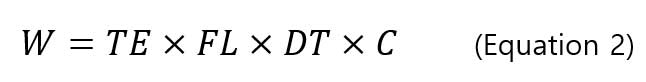
, where W is the particle mass (ng/event), TE is the transport efficiency (%), FL is the sample flow rate (mL/min), DT is the dwell time (min/event), and C is the mass concentration of analyte (ng/mL). Based on the calibration curve of signal intensity-dissolved mass concentration and the mass equation per particles-mass concentration, a calibration curve is constructed for signal intensity and mass per particle. Figure 5 shows an example of a corresponding calibration curve.
allows user to calculate particle mass by knowing the signal intensity using the following equation:
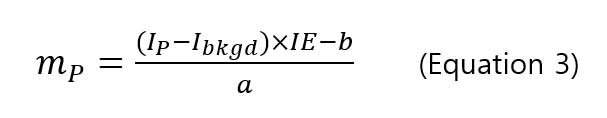
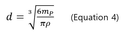
,where mPis the particle mass, IPis the signal intensity of particle,Ibkgd is the background intensity, IE is the ionization efficiency (%), a and b are the slope and y-intercept of intensity-mass of particle calibration curve. The ionization efficiency (IE) is 100% for silver and gold nanoparticles [8, 9, 10] with particle mass, and the diameter of particle can be calculated using the mass-diameter equation
In order to determine the transport efficiency (TE) of sp-ICP-MS, Pace and colleges suggested two methods: particle size method and particle frequency method (or particle concentration method). Both methods require a well-characterized reference nanoparticle sample.
The particle size method requires two calibration curves. One is the particle calibration curve and the other is dissolved ions calibration curve. Particle calibration curve is made by measuring sp-ICP-MS of well-characterized reference nanoparticle sample (i.e., the particles are spherical and have a narrow size distribution). The equation or particle calibration curve is:
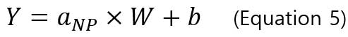
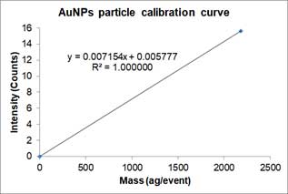
,where Y is the signal intensity (counts), W is the mass per event, b is the background noise of instrument, a_NP is the slope of calibration curve. Below is an example of a particle calibration curve measured at 60nm-AuNPs.
Dissolved ions calibration curves are made by measuring sp-ICP-MS of standard dissolved ion sample at different known concentrations and has a linear equation form as a particle calibration curve. Figure 7 shows an example of the dissolved calibration curve for gold ions.
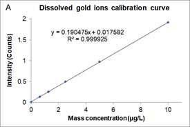
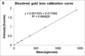
Figure 7A is the mass concentration dissolved calibration curve that correlates the mass concentration (μg/L) of dissolved gold ions with the intensity of instrument. Figure 7B is the converted calibration curve in which the mass concentration (μg/L) is converted to mass per event (ag/event) by multiplying each dissolved concentration by the sample flow rate and the dwell time. Compared with Equation 2, this transformation only considers the flow rate and dwell time, since the value of transport efficiency is not yet known. Thus, assuming that transport efficiency is the same for dissolve ions and nanoparticles, and calibration curves or dissolve ions (Figure 7B) and nanoparticles (Figure 6) should be equivalent. The y-intercept difference between the two calibration curves is negligible because it is the background intensity of the instrument. When converting the mass concentration calibration curve (Figure 7A) to mass per event calibration curve (Figure 7B), the slopes of the two calibration curves are different, because we the transport efficiency is not taken into account. The ratio between the two slopes of the calibration curve is the transport efficiency [8]:
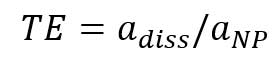
,where TE is transport efficiency, adiss is the slope of dissolved ions calibration (mass per event vs intensity), and aNP is the slope of particle calibration curve. Transport efficiency can be calculated from the slopes of dissolved gold ions calibration curve (Figure 7B) and the particle calibration curve (Figure 6):

In the particle concentration method, measure the pulse frequency (pulse/min) where the particle concentration is equal to the number of particles/min of the known nanoparticle suspension solution. The transport efficiency can be obtained by dividing the measured particle number by the total particle number of particles introduced into sp-ICP-MS instrument.
Limitations of sp-ICP-MS
The size limit of sp-ICP-MS is 10 nm to 2000 nm. The lower diameter limit is affected by the background/noise of the instrument. Cornelis and colleagues demonstrated the ability to measure 10 nm gold nanoparticles by deconvolution method to separate noise and signals from small nanoparticles [11]. The upper diameter limit is affected by the transport process. Previous studies [12, 13] showed that particles larger than 2um were removed from the spray chamber and could not reach the plasma. Therefore, the upper diameter limit of sp-ICP-MS for particles would be 2000 nm.
In addition, the mass spectrometer is used for the same measurement as the conventional ICP-MS, the sensitivity of the detector and the interference in the measurement depend greatly on the element to be analyzed.
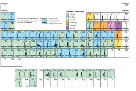
As shown in Figure 8, the detection limit varies with ionization efficiency and other factors. Analytes are separated by mass-to-charge, ratios, so interference occurs when the mass-to-charge ratio of an isobar or oxide is equal to the target element. For example, K and Ca are the same as Ar, Fe is ArO and Si, P, and S the are co-mass to charge ratios for CO, which causes large interference. Selecting isotopes avoids interference, but if choosing isotopes with low abundance can cause various problems, such as difficulty in obtaining a calibration curve. Therefore, in order to analyze the element with high interference, KED mode (Kinetic Energy Discrimination, using He gas) or DRC mode (Dynamic Reaction Cell, using NH3, O2, CH4 gas) is required for analyzing other gases in parallel. There is an appropriate mode depending on the element. For example, K and Ca causing interference by Ar, are meaningless to measure using KED mode and can only be analyzed using DRC mode using ammonia gas. In the case of sp-ICP-MS that deals with nanoparticles, when the target atom is small atomic mass, the number of particles increases with weight concentration (ppm, ppb, ppt). Therefore, the experimental conditions should be take into account, depending on the detection limit and the sensitivity of the detector.
References
- [1] Size distribution and concentration of inorganic nanoparticles in aqueous media via single particle inductively coupled plasma mass spectrometry, ISO/TS 19590 (2017).
- [2] ICP-MS measurement, S2nano Wiki, 27 Feb. 2017, http://nanowiki.s2nano.org/index.php/ICP-MS_measurement
- [3] Inductively coupled plasma mass spectrometry, Wikipedia, 24 Nov. 2019, https://en.wikipedia.org/wiki/Inductively_coupled_plasma_mass_spectrometry
- [4] Perkin Elmer, Standard Operating Procedure (SOP) - Single Cell Samples Analysis by NexION® 1000/2000, Draft 1.0 (2018).
- [5] C. Stephan, K. Neubauer, and C. T. Shelton, "Single Particle Inductively Coupled Plasma Mass Spectrometry: Understanding How and Why," PerkinElmer white paper (2014).
- [6] D. A. Skoog, F. J. Holler, and S. R. Crouch, Principles of instrumental analysis, Cengage learning (2017).
- [7] Perkin Elmer, The 30-Minute Guide to ICP-MS (2001).
- [8] H. E. Pace et al., "Determining transport efficiency for the purpose of counting and sizing nanoparticles via single particle inductively coupled plasma mass spectrometry,” Analytical chemistry 83, 9361-9369 (2011).
- [9] S. Hu et al., "A new strategy for highly sensitive immunoassay based on single-particle mode detection by inductively coupled plasma mass spectrometry," Journal of the American Society for Mass Spectrometry 20, 1096-1103 (2009).
- [10] F. Laborda et al., "Selective identification, characterization and determination of dissolved silver (I) and silver nanoparticles based on single particle detection by inductively coupled plasma mass spectrometry," Journal of Analytical Atomic Spectrometry 26, 1362-1371 (2011).
- [11] G. Cornelis and M. Hassellöv, "A signal deconvolution method to discriminate smaller nanoparticles in single particle ICP-MS," Journal of Analytical Atomic Spectrometry 29, 134-144 (2014).
- [12] L. Ebdon and A. R. Collier, "Particle size effects on kaolin slurry analysis by inductively coupled plasma-atomic emission spectrometry," Spectrochimica Acta Part B: Atomic Spectroscopy 43, 355-369 (1988).
- [13] P. Goodall, M. E. Foulkes, and L. Ebdon, "Slurry nebulization inductively coupled plasma spectrometry-the fundamental parameters discussed," Spectrochimica Acta Part B: Atomic Spectroscopy 48, 1563-1577 (1993).
Sample Preparation
Several standard solution sets are required to prepare for sp-ICP-MS measurements. To determine transport efficiency, dissolved ions calibration standard is required, which is a suspension solution of standard nanoparticles such as gold or silver nanoparticles. In order to measure samples of unknown size, it is necessary to know which elements need to be analyzed and prepare dissolved ions calibration standards or suspension solution of the standard nanoparticles of those elements.
Sample preparation transport efficiency
- 1.1. ample preparation for dissolved calibration curve
Prepare 0.625, 1.25, 2.5, 5 and 10 ng/mL Au dissolved solution from Au standard solution and use HCl 10 %/ HNO3 1 % as solvent.
- 1.2. Sample preparation for particle calibration curve
Prepare a suspension solution of 60 nm gold nanoparticles with a mass concentration of 0.25 ng/mL. Spherical gold nanoparticles can be purchased from nanoComposix (San Diego, USA).
Sample preparation to determine the size of unknown samples
- A. Sample preparation for dissolved calibration curve
Prepare a standard dissolved ions solution of the elements required for analysis. The concentration range can be 0.625 to 10 ng/mL. A series of standard dissolved ions solutions can be 0.625, 1.25, 2.5, 5 and 10 ng/mL.
- B. Sample preparation for particle calibration curve
Prepare a suspension of the components for analyzing. Select a particle size range that includes the size of the unknown sample to be measured. The concentration is 2x10⁷ particles/L (~ 50ng/L for gold 60nm particles and ~ 25ng/L for silver 60nm particles).
- C. Sample dilution
In general, to obtain useful results, the particle concentration of the sample to be measured should be between 2x10⁶ - 2x10⁸ particles/L. If there is no information about the particle concentration of the sample, it is recommended to dilute it 10000 times as a starting point. Use deionized water when diluting the sample. If stabilization is required, add sodium citrate or sodium dodecyl sulphate (SDS) to the deionized water at a concentration of 5 mM.
Measurement
Instrument Information
- 1. Instrument: PerkinElmer NexION 300D
- 2. S/W: Syngistix – Single Cell 1.2

Instrument Startup and Optimization
- a) Turn on the instrument.
- Turn on the cooler before starting the measurement.
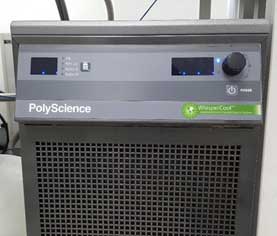
Figure 2. Cooler for ICP-MS instrument - Set the peristaltic pump tubing (sample inlet and outlet (drain waste) tubing).
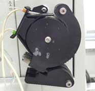
Figure 3. Peristaltic pump - Turn on the plasma.
In Syngistix software, select Syngistix tab, and then click the Control tab (Figure 4). In the Devices window, select the ICP-MS tab and click the Plasma button to turn on the Plasma (Figure 5) and wait for the Plasma button to change from Grey to Yellow to Green.
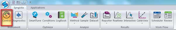
Figure 4. Syngistix software user interface. 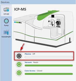
Figure 5. Plasma display. - Turn on the pump.
In the Devices window, select the Pump tab and the input pump speed (rpm). In later optimization step, the typical speed is -20 rpm (negative means counterclockwise direction). After the pump is turned on, the pump's input tube is placed in a deionized water 50mL tube for washing.
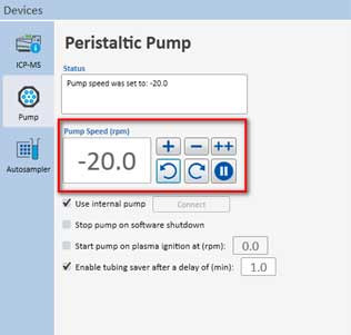
Figure 6. Pump speed setting
- Turn on the cooler before starting the measurement.
- b) Optimization for ICP-MS instrument
- Prepare 5 mL of NexION Setup Solution from Perkin Elmer (Figure 7) and inject this solution into the ICP-MS system by putting the input tube of the pump into this solution.

Figure 7. NexION setup solution from Perkin Elmer. - In the Syngistix software, select the Syngistix tab and click the SmartTune tab.
- Then select Smart Tune Manual and right click on [STD] Performance check and select Quick Optimize (Figure 8).
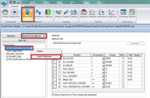
Figure 8. Optimization for ICP-MS. - After a Quick Optimize, the Results windows show passed/failed for the optimization. The result passed is shown in Figure 9. If the optimization failed, run Quick Optimize of [STD] Performance check again. If it still fails, check the Torch Alignment, Nebulizer Gas Flow, [STD/DRC] QID (Figure 8), by right clicking, select Quick Optimize, and check [STD] Performance Check again.
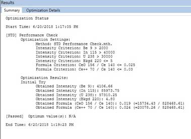
Figure 9. Passed result of Optimization. - Save the working conditions when the optimization has passed. In the Syngistix tab, select the Conditions tab (Figure 10), then click the upper left icon and select Save As (Figure 11). Save the conditions file to computer.
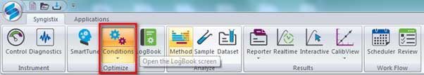
Figure 10. Select the Conditions tab in Syngistix software. 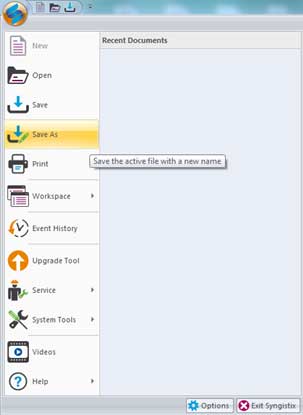
Figure 11. Save the working conditions in Syngistix software
- Prepare 5 mL of NexION Setup Solution from Perkin Elmer (Figure 7) and inject this solution into the ICP-MS system by putting the input tube of the pump into this solution.
Sample flow rate and transport efficiency determination
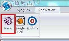
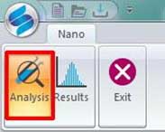
Click the Application tab and select Single Cell; in the Single Cell tab, select Analysis (Figure 12).
- a) Determine the sample flow rate.
- Set the pump speed to -10.0 rpm.
- Weigh using a 15 ml conical tube containing deionized water (record the value in g, this is m0).
- Insert the pump's input into the conical tube above the tube and record the time.
- After t minutes (typically 5-15 minutes), take the input from the pump and reweigh the conical tube to measure the weight m_1.
- Calculate the sample flow rate:

- After calculating the sample flow rate, enter this value into the software (TE tab and Sample tab as shown in Figure 13)
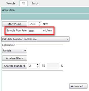
Figure 13. Enter sample flow rate on the TE (transport efficiency) tab. You need to enter this value again in the Sample tab.
- b) Determine the transport efficiency(TE).
- Move to TE tab as shown in Figure 13.
- Setting Parameters, Calibration, and Pump settings according to Figure 14-16.
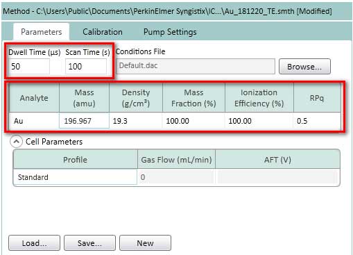
Figure 14. Setting Parameters for TE. The element analyzed here is gold (Au), but if there is a standard dissolved ion and nanoparticle suspension, user can choose another metal element. Typical value of dwell time is 50us. Typical values for Scan Time is 30-120s. 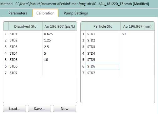
Figure 15. Calibration of settings for TE. In the left box, the dissolved ion concentration is 0.625 - 10 ug/L (or ng/mL). AuNPs 60 nm is chosen as the standard nanoparticles suspension (right box). 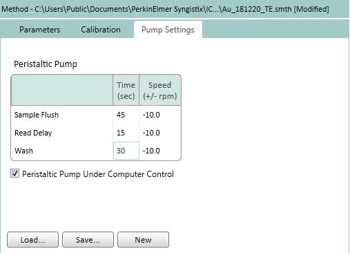
Figure 16. Set the Pump Settings on the TE. The Pump speed is kept constant (-10rpm) for Sample Flush (time to move from sample solution to plasma), Read Delay (delay detector time) and Wash (wash time after completing analysis of one sample). - On the TE tab, select how to determine the transport efficiency (based on particle size or particle concentration). This protocol uses a method based on particle size (Figure 17).
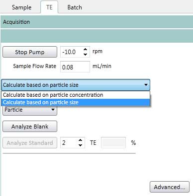
Figure 17. Select method based on particle size to determine the transport efficiency. - Measure standard solution of the dissolved ions calibration curve by selecting Dissolved (Figure 18) on the TE tab. Click Analyze Blank to measure a blank sample. Then click on Analyze Standard 1, 2, 3, 4, 5 one by one. After each measurement, the pump’s input is placed in deionized water for cleaning.
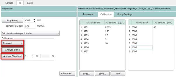
Figure 18. Measure standard solutions for dissolved ions calibration curve. - On the TE tab, select Particle (Figure 19) to measure standard solutions for particle calibration curve. Click Analyze Blank to measure a blank sample. Then click Analyze Standard 1.
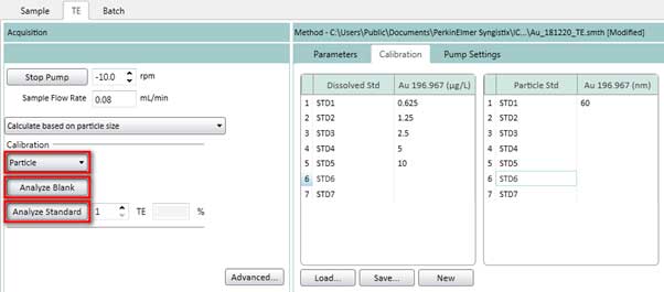
Figure 19. Measure standard solutions for particle calibration curve. - After completing the dissolved ions calibration curve and the particle calibration curve, the transport efficiency value is calculated and automatically entered into the TE box. The transport efficiency value depends on the chamber and the conditions used. 5-7% is ideal when using cyclonic chambers.
Measure unknown sample.
- a) Calibration curve
- Similar to section 4.3b, go to the Sample tab (Figure 20), setup Parameters, Calibration and Pump Settings (Figure 14 - 16). The Pump Settings should be same as the TE step in Figure 16. Figure 20 shows an example of gold element setting. The setting for other elements such as silver can be done in the same way.
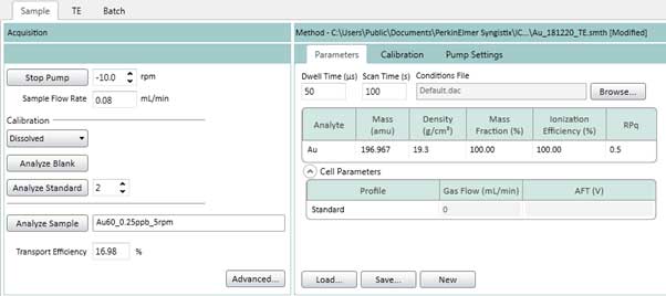
Figure 20. Sample tab settings (element is gold). 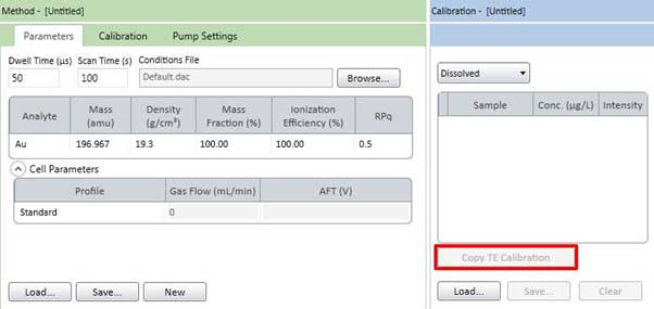
Figure 20-1. Copy the calibration curve from the TE tab. - If the component of the sample to be measured is the same as the material used to determine the transport efficiency, the calibration curve used for the transport efficiency can be reused on the sample tab. To copy a calibration curve, press the Copy TE Calibration button in Figure 20-1. At this point, you need to select and copy Dissolved and Particle.
- From the Calibration of the Sample tab (Figure 20), select Dissolved to construct a dissolved ions calibration curve, then click Analyze Blank to measure a blank sample. Then, select Analyze Standards 1, 2, … to measure standard solution. After completing all the standard solutions, a calibration curve is generated. This curve is used to measure samples of unknown size.
- If you have standard nanoparticles of the component you want to analyze, you can draw a particle calibration curve by selecting Particles in the calibration box in Figure 20. The particle calibration curve is constructed by measuring the background sample and the standard solution in the same way as when constructing the ion calibration curve.
- Only dissolved ions calibration curve or particle calibration curve can be used.
- Similar to section 4.3b, go to the Sample tab (Figure 20), setup Parameters, Calibration and Pump Settings (Figure 14 - 16). The Pump Settings should be same as the TE step in Figure 16. Figure 20 shows an example of gold element setting. The setting for other elements such as silver can be done in the same way.
- b) Measurement sample of unknown
- Enter a sample name in the box next to Analyze Sample button (Figure 20).
- Put the pump input into a sample of unknown size, then click Analyze Sample.
- After completing the sample of unknown size, put the input of the pump back into the deionized water.
Maintenance and Daily Turn-Off
After all measurements, increase the pump speed to -20 rpm and place the input of the pump into a 5 mL rinse solution (HNO3 1%).
After washing for 10 minutes with a rinse solution, the input from the pump is placed in a 5 mL deionized water tube.
After 10 minutes of washing with deionized water, wait 2-3 minutes to rinse off all the liquid inside the pump tubes, then turn off the Plasma (use the same button in the Syngistix Control windows - Figure 12).
After turning the plasma for 15 minutes, turn on the cooler system.
Exporting data
- After completing the sample measurement, go to the Results tab to see the results.
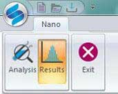
Figure 21. Results tab for viewing results. 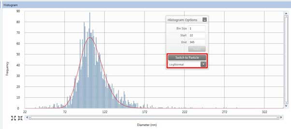
Figure 22. Histogram of the Results tab. - The histogram box (Figure 22) on the Results tab shows sample measurement results. In the Histogram Options window, click Switch to Particle/Switch to Dissolved to display the results of converting the measured signal to particle size using the particle calibration curve/ion calibration curve. Depending on the shape of the histogram, you can select LogNormal, Gaussian, or Max intensity to see different modes depending on the selected option (This option has the same effect when measuring to obtain a calibration curve. Therefore, the user must select the appropriate curve fit).
- Select one measurement in the Results Table windows (Figure 23), then click the Export button in File Options windows (Figure 24) and save the data as an Excel (.xlsx) file.
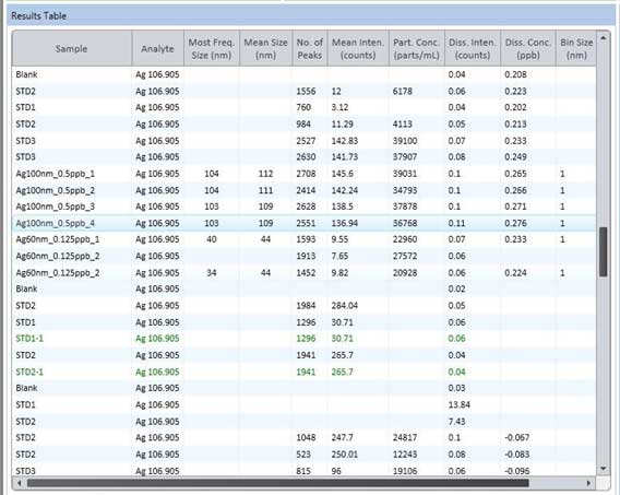
Figure 23. Result table of sp-ICP-MS. 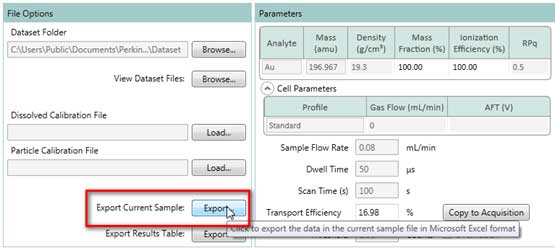
Figure 24. Export data to Excel file.
Data Processing & Analysis
Excel files exported from Syngistix software are used to collect data from nanoparticle samples.
Excel file has 4 sheets:
Sample Information, Size Histograms, Intensity Histograms, and Calibrations.
- 1. Sample Information sheet contains information about the sample (name, element, density, particle count, mean size, particle concentration, etc.) and the instrument (flow rate, transport efficiency).
- 2. Size Histogram sheet contains frequency information of each calculated size and fitting (Gaussian, Lognormal, Max Intensity) for sample.
- 3. Intensity Histogram contains the frequency information of each intensity (i.e. the intensity of each particle).
- 4. Calibrations sheet contains calibration curve information related to the mass (size) per particle and intensity.