Laboratory
-
DLS Principle
-
DLS Sample Prep.
-
DLS Measurement
-
DLS Data Analysis
Summary of Analytical Technique
Dynamic Light Scattering (DLS) is one of the most commonly used techniques for size determination of nanoparticles (NPs) in suspension solution. DLS determines hydrodynamic size of the NPs in the suspension by measuring fluctuating intensities of scattered light induced by the Brownian motion of the NPs. Depending on the refractive index and structure of the NPs, DLS can theoretically measure NPs with hydrodynamic size in the range of 0.3 nm - 10 um, but usually NPs with a hydrodynamic size between 2 – 3,000 nm is recommended[1]. Concentration of samples in DLS measurements is about 108 – 1012 particles per mL which can be up to 1000 times higher than concentration of samples in another scattering based method - Nanoparticle Tracking Analysis (NTA)[8]. Theoretically, DLS is able to resolve particles in mixture when their diameters ratio is 1:3 (i.e. 100 nm particles can be resolved from 300 nm particles). In practice, that ratio is 1:4. In comparison with the NTA technique, DLS can measure hydrodynamic sizes of NPs in a wider size range, higher concentration range, and lower size resolution[1]. Additionally, the intensity of scattered light is related to the refractive index of the NPs and proportion to the sixth power of the diameter. Hence, DLS is sensitive to impurities, especially large particles with high refractive indices, and is not suitable for measuring samples containing other interfering NPs.
Principle of Analytical Technique
DLS is used to measure the hydrodynamic size of the particles in suspension solutions. The particles undergo Brownian motion at different velocities in the suspension depending on their size. The variation of scattered laser beam by these particles is measured over time. This intensity fluctuation of laser light can be used to analyze the hydrodynamic size of a particle from its correlation function of intensity fluctuations (small particles have faster Brownian motion than large particles, so the correlation function decreases faster). The diffusion coefficient can be determined by measuring the decreasing rate of the correlation function according to the size of particles. The hydrodynamic diameter of a particle can be calculated by substituting the value of diffusion coefficient into the Stokes-Einstein equation .
![Figure 1. Correlation function (image from [DLS Measurement, http://nanowiki.s2nano.org/index.php/DLS_measurement])](/img/contents/Laboratory/dls/img_dls_01.jpg)
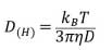 Stokes-Einstein equation
The Stokes-Einstein equation, where D(H) is the hydrodynamic diameter, kB is the Boltzmann constant, T is the absolute temperature, η is the viscosity, and D is the diffusion coefficient. The particle diffusion coefficient is obtained through the reduction rate of the correlation function and the spherical hydrodynamic diameter is derived from the above equation. Therefore, an error may occur if the sample is not spherical.
References
- [1] S.K. Brar and M. Verma, “Measurement of Nanoparticles by Light-scattering Techniques,” TrAC Trends in Analytical Chemistry 30, 4-17 (2011).
- [2] “What is the maximum viscosity for DLS?,” Materials Talks, www.materials-talks.com/blog/2017/09/26/what-is-the-maximum-viscosity-for-dls/,
- [3] DLS Measurement, S2nano Wiki, http://nanowiki.s2nano.org/index.php/DLS_measurement
- [4] Particle Size Analysis-Dynamic Light Scattering (DLS), ISO 22412 (Wsitzerland, Geneva, 2017).
- [5] S. M. Briffa, I. Lynch, and E. Valsami-Jones, “Characterisation of NMs by Means of DLS,” NanoMILE Scientific Protocol (2017).
- [6] K. A. Jensen, “NRCWE SOP for Measurement of Hydrodynamic Size Distribution and Dispersion Stability by Dynamic Light Scattering (DLS),” National Research Centre for the Working Environment (2015).
- [7] Malvern Panalytical, Zeta Potential & Particle Size Analyzer User Training Manual (2018).
- [8] V. Filipe, A. Hawe, and W. Jiskoot, “Critical Evaluation of Nanoparticle Tracking Analysis (NTA) by NanoSight for the Measurement of Nanoparticles and Protein Aggregates,” Pharmaceutical Research 27, 5 (2010).
Sample Preparation
Solid powder
- 1. Add powder to solvent (DI water, toluene, etc.). See Table 2 below for proper concentration.
- 2. Disperse the sample for 5-15 minutes using a sonicator
Liquid suspension
- 1. Dilute the sample in solvent (DI water, toluene…).
- 2. Mix using a vortexer.
Cautions
- - The particles should be well dispersed in the solution.
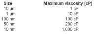
- - The viscosity of the solvent should not be too large to interfere with Brownian motion of the particles. The viscosity limits of the solvent according to the particle size in the DLS measurement are shown in the table below[2].
- Sample volume should be at least 2mL.
- The diameter of the sample for DLS measurement is preferably in the range of 2-3000nm[1].
- The sample should be free of air bubbles or dust in the solution. In particular, in the case of in vitro medium sample solution, care must be taken because the solution itself causes bubbles.
- Sample concentration for measurement depends on the characteristic of the sample.
- If the concentration of the sample is too low, insufficient scattering may occur in the measurement. This can be caused by a low particle mass fractions or the particle size distribution can be very wide. If the concentration is too high, multiple scattering may occur in addition to the scattered light due to one particle. In addition, if the particle is polydisperse(particle size difference is large), the signal intensity becomes very large and the scattering signal of small particles can be masked by the scattering signal of large particles. Therefore, for unknown samples, it is recommended to dilute the sample and measure it several times according to the concentration in order to obtain accurate results. Typically, the concentration of nanoparticles sample is appropriate at 0.01 - 0.5 mg/mL.
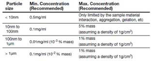
Table 2. Proper concentration condition according to particle size[7]. - No significant sedimentation of the sample should occur. If the sample has a large sedimentation after the measurement, it is necessary to reconsider whether the particle size is suitable for DLS.
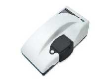
- Sample container (cell) is shown in Figure 1. Because the laser passes through the transparent side of the cell during measurement, the presence of fingerprints, oil, or dust on the cell surface can cause the measurement to fail. Therefore, when you grab a cell, hold the top of the cell, not the side of the cell.
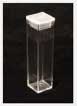
Figure 1. Sample Container – Cell (image from Malvern Panalytical).
Measurement
Instrument Information
- 1. Instrument: Malvern Zetasizer Nano – ZS90
- 2. S/W: Zetasizer Software version 7.10
Instrumental setting for Setting
- 1. Turn on instrument.
- i. Turn on power button behind the instrument.
- ii. Wait at least 5 minutes for the laser source to stabilize.
- iii. Press the round button which has red-green LED indicator to open the measuring chamber lid and insert the sample cell into the sample holder.
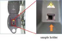
Figure 2. Sample holder. - 2. Open the Zetasizer Software.
- 3. Create a new measurement file(choose i or i or iii).
- i. File → New → Measurement File
- ii. Or Ctrl + N
- iii. Or Click the symbol

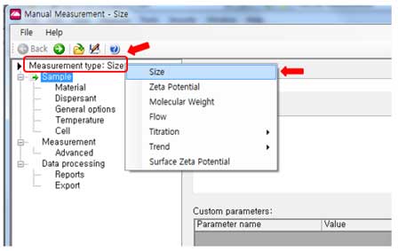
- 4. Choose Size.
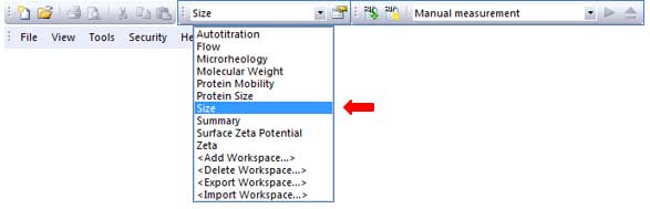
Figure 3. Zetasizer Software user interface-> Choose Size. - 5. Choose Manual measurement.
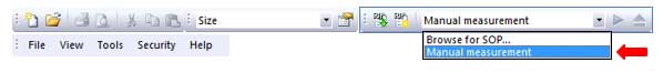
- 6. Click the measure button (green):
- 7. When the measurement setting window appears, proceed with the setting:
- i. Measurement Type: Choose the Size
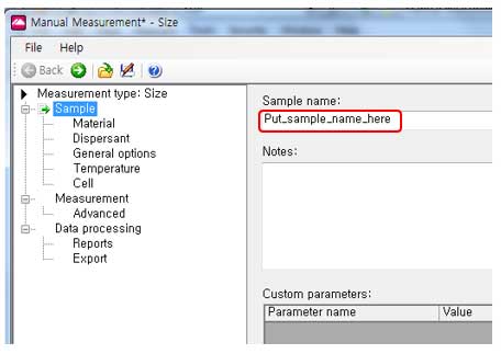
- Sample:
ii. Set a sample name. The sample name may include sample type, manufacturing size, solvent, and time.
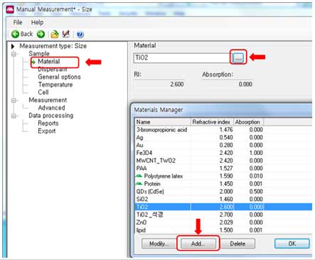
- Material:
iii. Select a material. Some materials are already defined in the software. If the material to be measured is not in the software list, the refractive index and absorption should be added to the list using the “Add” button.
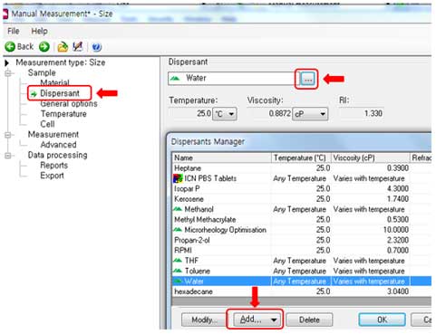
- Dispersant:
iv. Select a dispersant for solvent setting. Some solvents with specific temperature and viscosity are already defined in the software. If the solvent you are using is not in the software list, you can add viscosity at a specific temperature using the “Add” button.
- General options:
v. Leave it to default.
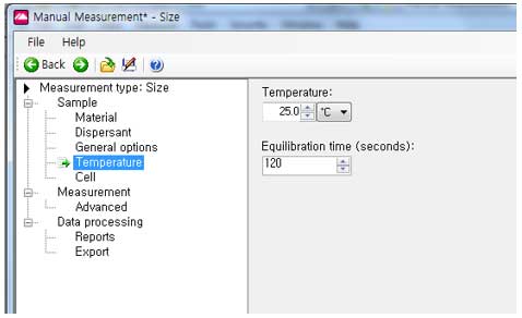
- Temperature:
vi. Set the measurement temperature (generally at room temperature-25℃). Select Equilibrium time(the equilibrium time is the time to stabilize the sample temperature and is set to 120 seconds by default; user can change this values, for example 30s, typical value is 30s).
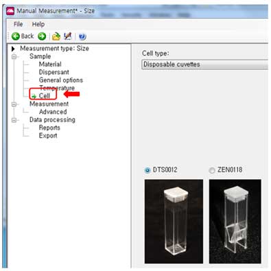
- Cell:
Select cell type (cuvette, typical cuvette is DTS0012).
vii. The cuvette DTS0012 is suitable for large sample volume (> 2mL). The cuvette ZEN0118 is used when the sample volume is small (approx. 50uL).
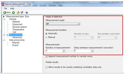
- viii. Settings for Measurement.
- a. Measuring angles: 90° (scattering signal)
- Measuring duration(Automatic):
b. Setting the measurement duration affects the accuracy and repeatability of the results. For Automatic setting, the software automatically determines the appropriate duration time. Most samples are left as default. The automatic measurement is divided into a minimum of 10 seconds.
- c. Measuring duration(Manual):
Set the duration time between 1 and 600 seconds. Be careful not to set the time too long because the measurement time is too long and may cause sedimentation.
- d. Number of measurements:
Normally 3 times. Set 10 times if you want an accurate measurement (depending on sample or situation). However, in this case, it is necessary to be able to distinguish abnormal results because there are many repeated analysis times.
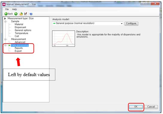
- ix. Data processing: Data processing is left to default.
- x. Finally, click the OK button:
- i. Measurement Type: Choose the Size
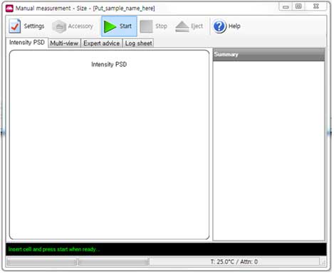
- 8. When the setting is completed, the measurement window appears
- 9. Click the Start button to perform the measurement
Cautions
Make sure that the there is no excessive ambient vibration during the measurement.
Results
After the measurement, select the measured data in the Records View and check the Quality Report. The Attenuator index of good measurements is lower than 11 and greater than 0. In addition, PdI (Polydispersity) index must be less than 1.000.
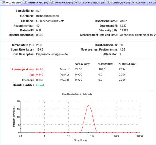
- I. Attenuator: measure the transmittance of the laser through the sample (0 ≤ attenuator ≤ 11). Attenuator=0 indicates that the entire laser beam is blocked (too diluted sample). Attenuator=11 means transmit 100% laser beam (sample concentration too low).
- II. Z-average: mean size of particles based on intensity.
- III. PdI: Polydispersity index – width of the size distribution (depending on intensity). PdI should be less than 1.000 and samples larger than 1.000 may not be suitable for DLS measurements.
- IV. 5 (Size quality report tab) shows an example of good DLS data.
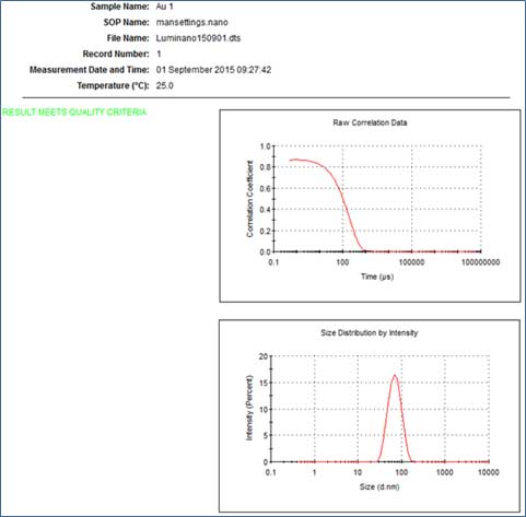
- V. If the phrase "Refer to quality report" appears in the Result quality, you need to analyze the sample further. Check the Size-distribution report and Expert advice to see if the large PdI is caused by polymodal distribution, dust, cuvette, large particles or sediment.
- VI. If parameters such as refractive index, absorption coefficient, or viscosity are not entered correctly in the measurement, they can be changed by clicking Edit → Edit Result in the program.
Data Processing & Analysis
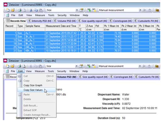
- 1. To export data, select the rows you want to export, then click the Intensity PSD tab or the Volume PSD tab (depending on what you want to analyze).
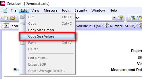
- 2. Select Edit→ Copy Size Values
- 3. Paste the results into Excel. This data can be used to draw a hydrodynamic size histogram. The figure below shows the data after copying and pasting into Excel. Column A is used as the X-axis (Hydrodynamic Diameter) and column B is used as the Y-axis (Intensity) to draw the graph in Excel.
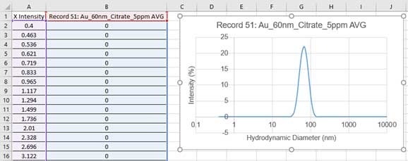
- 4. If you select data from multiple measurements (0s, 5s, 10s, 1min etc.), you can use the sigmaplt software to obtain the following contour plots (showing changes in hydrodynamic size over time):
- I. Select the data as shown below and click the Intensity, Volume, or Number:
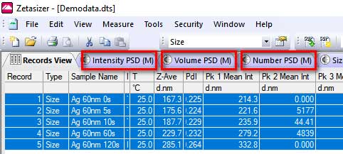
Figure 1. Data from multiple measurements. - ii. Choose Edit → Copy Size Values:
- iii. Run the Sigmaplot software and paste the results. The following figure shows sample data. Column 1 is hydrodynamic diameter and columns 2-6 are sample data for 0s, 5s, 10s, 60s and 120s.
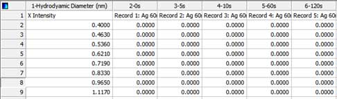
Figure 2. Results in Sigmaplot window. - Arrange the data in the following format:
Column 1 is time and column 2 is hydrodynamic diameter; they are fixed. Column 2 in figure 2 is transformed to Row 1 in figure 3. Column 3 in figure 2 is transformed to Row 2 in figure 3.
Column 4 in figure 2 is transformed to Row 3 in figure 3. Column 5 in figure 2 is transformed to Row 4 in figure iv. Column 6 in figure iii is transformed to Row 5 in figure iv.
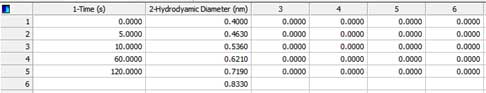
Figure 3. Arranged data. - v. After selecting all the data in section iv is selected, choose Graph→Create Graph→Contour Plot→Filled Contour Plot→ XY many Z→Finish. Now you can get the following Contour plot (Y-axis is Log scale):
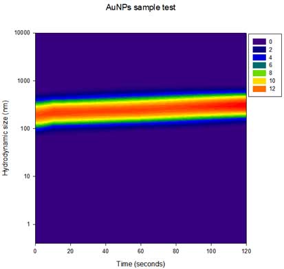
Figure 4. Contour plot for AuNP sample.
- I. Select the data as shown below and click the Intensity, Volume, or Number:
- 5. Create a report. The report should include the following information:
- i. Measurement date
- ii. Experimenter
- iii. Sample information: sample name, product number, etc.
- iv. Dispersion solvent
- v. Sample preparation method
- vi. Mean and standard deviation of the measured hydrodynamic size and size distribution of the particles.
- vii. Unusual characteristics that affect testing during measurement and analysis